The Sloan Digital Sky Survey (SDSS) is one of the greatest deep-sky surveys ever made. It has been launched by *Apache Point Observatory* in New Mexico, United States. Here, I’m going to introduce briefly some basic concepts needed to work with the rest of our tutorial. For a complete description, visit SDSS website.
SDSS sky coverage
Each survey has its own sky coverage. While some surveys may cover the full sky, most surveys cover only a part of the sky. Of course a telescope based on a certain location on the Earth can not see the whole sky. One possibility to find the coverage of surveys is to use the CDS MOCServer. We want to find if there are any MOCs (Multi-Order Coverage maps) related to the SDSS data releases. The astroquery.cds package has made this really simple:
from astroquery.cds import cds
import astropy.units as u

tbl = cds.find_datasets(meta_data='ID=*sdss*', fields=['ID'])

print(tbl)
               ID
--------------------------------
                CDS/II/259/sdss3
                CDS/II/267/sdss4
                CDS/II/276/sdss5
                CDS/II/282/sdss6
                CDS/II/294/sdss7
                CDS/II/306/sdss8
        CDS/J/A+A/544/A81/snsdss
     CDS/J/A+A/569/A124/guv_sdss
     CDS/J/A+A/597/A134/psb_sdss
         CDS/J/AJ/143/52/sdss_cl
                             ...
sdss.jhu/services/siapdr4-images
sdss.jhu/services/siapdr5-images
sdss.jhu/services/siapdr7-images
sdss.jhu/services/siapdr8-images
sdss.jhu/services/siapdr9-images
      wfau.roe.ac.uk/sdssdr3-dsa
      wfau.roe.ac.uk/sdssdr5-dsa
      wfau.roe.ac.uk/sdssdr6-dsa
      wfau.roe.ac.uk/sdssdr7-dsa
      wfau.roe.ac.uk/sdssdr8-dsa
      wfau.roe.ac.uk/sdssdr9-dsa
Length = 98 rows
It has found 98 MOCs. Let’s take the example of the data release 6 and download the corresponding MOC. The find_datasets function retrieve the requested data from the MOCServer. If you set the argument return_moc to True, the function will return the data as a MOC object. Note that we should pass the ID to the meta_data argument.
moc = cds.find_datasets(meta_data='CDS/II/282/sdss6',
                        return_moc=True)
Now, if you want to find if a certain point is covered by the returned MOC, you can simply pass it to the contains method. Let’s see if the following points have been covered in the SDSS sixth data release or not.
print(moc.contains(ra=0*u.deg, dec=0*u.deg))
print(moc.contains(ra=10*u.deg, dec=80*u.deg))
[ True]
[False]
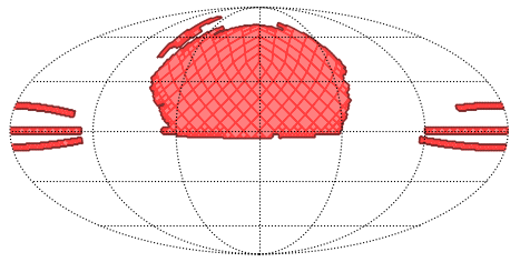
So, we can see that the first point is in the coverage but the second one is not. To plot the coverage of the MOC, we should use the mocpy package. I will write another post about it in the future, but for now let’s just see what the following code gives us.
import matplotlib.pyplot as plt
from astropy.coordinates import SkyCoord, Angle
from mocpy import World2ScreenMPL

fig = plt.figure(111)

wcs = World2ScreenMPL(fig=fig,
                      fov=360*u.deg,
                      center=SkyCoord(180, 0, unit='deg'),
                      coordsys="icrs",
                      rotation=Angle(0, u.deg),
                      projection="MOL" #AIT
                      ).w

ax = fig.add_subplot(1, 1, 1, projection=wcs)

moc.fill(ax=ax, wcs=wcs, alpha=0.5, fill=True, color="red")
moc.border(ax=ax, wcs=wcs, alpha=0.5, color="black")

plt.grid(color="black", linestyle="dotted")
plt.show()
The most basic types of data collected by the SDSS are photometric and spectroscopic data. In this article we only talk about these two types.
Photometric data
The photometric data is collected by a special type of camera that is equipped with 30 CCDs arranged in six columns and five rows.
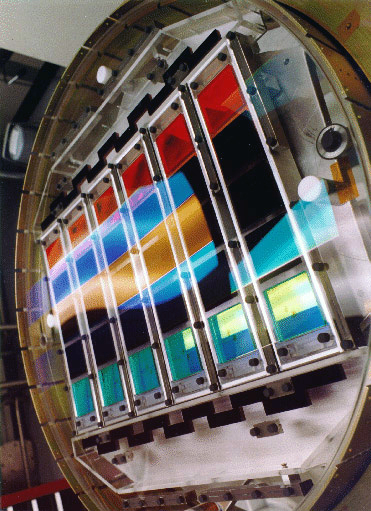
Each row of the camera uses a different filter. The center wavelengths of these filters are presented in table below. For a better understanding, you can compare them with the wavelengths of the visible light.
| NAME | u | g | r | i | z |
|---|---|---|---|---|---|
| COLOR | Ultraviolet | Green | Red | Near-Infrared | Infrared |
| WAVELENGTH | 3543 | 4770 | 6231 | 7625 | 9134 |

The process of scanning the sky occurs with very slow movement of the camera along its columns. Therefore, the CCDs in each column capture the same image but in five different filters.
Photometric data terminology
A strip is a scan along a line of constant survey latitude. The fraction of a strip observed at one time is a run. A camcol (camera column) is the output of one camera column of CCDs as part of a Run. A field is a part of a camcol that is processed by the Photo pipeline at one time. Fields are 2048 × 1489 pixels; a field consists of the frames in the 5 filters for the same part of the sky. For a brief description see here and for a more technical description see here.
If you have run, camcol and field of an image, you can see it via a tool called Get Fields. But we may not always know these parameters.
The SDSS team has assigned a unique ID to each object in the sky called ObjID. If you know already the ObjID of an object, you can easily find some of the parameters mentioned above using decode_objid function. For example, we want to find the parameters of an object whose ObjID is 1237648720693755918:
import sdss
dc = sdss.decode_objid(1237648720693755918)
print(dc)
{'version': 2,
 'rerun': 301,
 'run': 756,
 'camcol': 2,
 'first_field': 0,
 'field': 427,
 'id_within_field': 14}
Querying photometric data
All types of data are stored in a database is SDSS server. Although there are several web-based tools to access data, the most efficient way, sometimes the only way, is to use SQL query. You can type your query in the SQL Search page directly, or in a pythonic way, you can use the sql2df function from the sdss python package. Anyway, you should use the Schema Browser to find tables from which you want to retrieve data and their columns.
The photometric data are essencially stored in a table called PhotoObj. As an example, imagine that you want to find IDs, coordinates, types and magnitudes of objects whose apparent magnitude in g-band is between 0 and 6:
SELECT objID, ra, dec, type, u, g, r, i, z
FROM PhotoObj
WHERE g BETWEEN 0 AND 6
Since most of the SDSS targets have very high magnitudes (even higher than 20), the above query will return only 12 rows. But be careful when asking for huge data! I will show you how big is this database. You can use, for instance, TOP 10 to limit maximum number of rows returned up to 10.
SELECT TOP 10 objID, ra, dec, type, u, g, r, i, z
FROM PhotoObj
Now, let’s see how many objects are there in the PhotoObj table. We use sql2df function from sdss python package. This function accepts a SQL query as string and returns a pandas DataFrame.
sql = "SELECT COUNT(*) AS num_obj FROM PhotoObj"
df = sdss.sql2df(sql)
print(df)
     num_obj
0  794328715
You can see that there are about 800 million objects in this table! This is really huge. What are these objects? To find out, we should look at type column of the table. Let’s see how many groups exist and how many objects belong to each group.
sql = """
SELECT COUNT(*) AS num_obj, type
FROM PhotoObj
GROUP BY type
"""

df = sdss.sql2df(sql)
print(df)
     num_obj type
0      50229    0
1  366339137    3
2  427939349    6
As you see in the results, there are three types: 0, 3 and 6. These are value codes: 0 for UNKNOWN, 3 for GALAXY, 6 for STAR. So, it seems that most of the objects are stars. But this is just a classification based on the photometric data. It can be incorrect since the photometric data of a star and a quasar could be similar. For a more accurate classification we need the spectrum of an object. We will discuss this later.
For now, let’s recode our DataFrame by replacing the value codes with the names of each type and then calculate the percentage of each type. But before, we need to convert the data types of the columns of our DataFrame (which are initially str) to int.
df = df.astype(int)
df.loc[df['type']==0, 'type'] = 'UNKNOWN'
df.loc[df['type']==3, 'type'] = 'GALAXY'
df.loc[df['type']==6, 'type'] = 'STAR'
df['percent'] = 100 * df['num_obj'] / df['num_obj'].sum()
print(df)
     num_obj     type    percent
0      50229  UNKNOWN   0.006323
1  366339137   GALAXY  46.119337
2  427939349     STAR  53.874340
Now, it’s easier to see that about %46 of objects are of type GALAXY, and about %54 of objects are of type STAR.
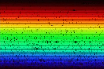
Spectroscopic data
SDSS collects two major types of spectra: one-dimensional and two-dimensional. Here, I’m going to talk about the 1D spectra.
The spectrum of an object can be identified with three numbers: Plate, MJD and FiberID. The reason behind these numbers is that the SDSS records spectra using aluminum plates placed at focal plane of the telescope. Each plate has a unique plate number and it is connected to the spectroscope via 1000 optical fibers. Each optical fiber transmits the light of one object to the spectroscope and is identified by a unique fiber_id. The date at which the spectrum has been recorded is identified with mjd, which is the Modified Julian Date.
Another way that SDSS identifies the spectrum of an object is by an identifier number, called SpecObjID. If you know SpecObjID of an object, you can find the above mentioned parameters using decode_specid function of sdss python library:
dc = sdss.decode_specid(320932083365079040)
print(dc)
{'plate': 285, 'fiber_id': 184, 'mjd': 51930, 'run2d': 26}
Note that SpecObjID is different from ObjID. We should use ObjID when we need the photometric data of an object, and SpecObjID for spectrometric data. In fact, the number of photometric objects are much higher than spectrometric objects. It means that for most of the objects, there is no spectrometric data. We will discuss this later.
Querying spectroscopic data
The spectroscopic data is essetially stored in SpecObj table of SDSS database. Let’s say we want to retrieve specObjID, ObjID, mjd, plate, fiberID and z (redshift) for the first five rows of this table. In this table, ObjID is stored as bestObjID column name.
sql = """SELECT TOP 5
specObjID, bestObjID, mjd, plate, fiberID, z
FROM SpecObj"""

df = sdss.sql2df(sql)
print(df)
             specObjID            bestObjID    mjd plate fiberID              z
0  3154868093696632832  1237663268796432489  54326  2802     351  -0.0001514952
1  3154870567597795328  1237663268796432699  54326  2802     360  -6.223064E-05
2  3154870017841981440  1237663268796497989  54326  2802     358  -8.696781E-05
3  3154868918330353664  1237663268796498001  54326  2802     354  -0.0003906398
4  3154866719307098112  1237663268796498065  54326  2802     346   -0.000104708
As another example let’s find out how many spectroscopic object are in this table and the spectroscopic class each object belongs to.
sql = """
SELECT COUNT(*) AS num_sp, class FROM SpecObj
GROUP BY class
"""

df = sdss.sql2df(sql)
df['num_sp'] = df['num_sp'].astype(int)
df['percent'] = 100 * df['num_sp'] / df['num_sp'].sum()
print(df)
    num_sp   class    percent
0  2963274  GALAXY  58.023260
1  1102641     QSO  21.590587
2  1041130    STAR  20.386153
As you see, the are more than five million spectroscopic object in this table. Most of these objects are galaxies, while about %22 are quasars and %20 are stars. Now let’s find how many object exist in large redshift, for example at z greater than 1:
sql = """
SELECT COUNT(*) AS num_sp, class FROM SpecObj
WHERE z>1
GROUP BY class
"""

df = sdss.sql2df(sql)
df['num_sp'] = df['num_sp'].astype(int)
df['percent'] = 100 * df['num_sp'] / df['num_sp'].sum()
print(df)
   num_sp   class    percent
0   75462  GALAXY   8.018174
1  865675     QSO  91.981826
As you see, about %92 of spectral objects whose redshifts are greater than one are quasars. This is really interesting because we know that quasars do not exist any more!
Region
You can select a region in the sky with sdss.region class by passing coordinates of its center. There are some optional arguments you can pass to this class: fov, width, heigth, opt and query. The fov argument is the field of view in degrees and the opt argument has been explained here.
ra = 179.689293428354
dec = -0.454379056007667
reg = sdss.Region(ra, dec, fov=0.1, opt='')
reg.show(figsize=(8,8))

Instead of show you can use show3b to get the image in the three filters.
reg.show3b(figsize=(15,8))

The region class has some useful methods and attributes, such as: the .data attribute which gives you the image data; the .nearest_objects() and the .nearest_spects(), which give you dataframes of photo objects and spectro objects in the region.
df_obj = reg.nearest_objects()
df_sp = reg.nearest_spects()
print(df_obj.shape)
print(df_sp.shape)
print(df_sp)
(329, 11)
(4, 15)
                 objID            specObjID  ...      zErr  zWarning
0  1237648720693755918   320932083365079040  ...  0.000016         0
1  1237648720693690602   320942253847635968  ...  0.000021         0
2  1237648720693690487  4326862017850003456  ...  0.000007         0
3  1237674649928532213  3284333942458574848  ...  0.000007         0

[4 rows x 15 columns]
We will write about more advanced features of SDSS in the future posts.