The spectrum of an object can give us a lot of information, such as type of the object, radial velocity, redshift, presence of chemical elements or compounds in its atmosphere, an estimate of its distance, etc. In this article we take a look at one-dimensional spectra created by SDSS and saved in FITS files.
I suppose the reader has at least some basic knowledge about spectroscopy, redshift, SDSS and FITS files. If this is not the case, you can refer to:
Inspecting the spectrum in a FITS file
I have already explained in another post, three different methods to download the spectrum of an object from SDSS servers. By creating an instance of the SpecObj class from the sdss python package and passing the specObjID, you can download the spectrum as a FITS file by calling the download_spec method:
import sdss

sp = sdss.SpecObj(320932083365079040)

sp.download_spec()
Now, we have a file named spec-0285-51930-0184.fits in our working directory. A good option to handle FITS files is using astropy.io.fits package. Let’s import the neccessary libraries and open the downloaded file.
import numpy as np
import pandas as pd
import matplotlib.pyplot as plt
from astropy.io import fits
from astropy import units as u

hdul = fits.open('spec-0285-51930-0184.fits')
hdul.info()
Filename: spec-0285-51930-0184.fits
No.    Name      Ver    Type      Cards   Dimensions   Format
  0  PRIMARY       1 PrimaryHDU     142   ()
  1  COADD         1 BinTableHDU     26   3839R x 8C   [E, E, E, J, J, E, E, E]
  2  SPECOBJ       1 BinTableHDU    262   1R x 126C   [6A, 4A, 16A, 23A, 16A, 8A, E, E, E, J, E, E, J, B, B, B, B, B, B, J, 22A, 19A, 19A, 22A, 19A, I, 3A, 3A, 1A, J, D, D, D, E, E, 19A, 8A, J, J, J, J, K, K, J, J, J, J, J, J, K, K, K, K, I, J, J, J, J, 5J, D, D, 6A, 21A, E, E, E, J, E, 24A, 10J, J, 10E, E, E, E, E, E, E, J, E, E, E, J, E, 5E, E, 10E, 10E, 10E, 5E, 5E, 5E, 5E, 5E, J, J, E, E, E, E, E, E, 25A, 21A, 10A, E, E, E, E, E, E, E, E, J, E, E, J, 1A, 1A, E, E, J, J, 1A, 5E, 5E]
  3  SPZLINE       1 BinTableHDU     48   29R x 19C   [J, J, J, 13A, D, E, E, E, E, E, E, E, E, E, E, J, J, E, E]
The fits.open function returns an HDUList object. We used the info method of this object to view the summarized content of our file. As you see in the above results, the FITS file consists of a primary HDU (hdul[0]) and three extensions (hdul[1], hdul[2], hdul[3]). The primary HDU contains only the Header keywords. The three extensions are of type BinTableHDU, each of them with its own header and data.
To see the column names of each table, use the columns attribute. Wavelength and flux of the spectrum are stored in the first extension (hdul[1]). Let’s see all columns of this extension:
cols1 = hdul[1].columns
print(cols1)
ColDefs(
    name = 'flux'; format = 'E'
    name = 'loglam'; format = 'E'
    name = 'ivar'; format = 'E'
    name = 'and_mask'; format = 'J'
    name = 'or_mask'; format = 'J'
    name = 'wdisp'; format = 'E'
    name = 'sky'; format = 'E'
    name = 'model'; format = 'E'
)
The wavelengths are stored in the loglam column in the logarithmic scale. The flux column is the raw flux data as recorded by the spectroscope, and the model column is the result of the best fitted model on the flux. In most cases we prefer to use model instead of flux.
To access the data stored in each extension, we should first use the data attribute. Then we can access values of each columns by using field method and passing the column name. Let’s extract wavelength, flux and model columns:
data1 = hdul[1].data

wavelength = 10 ** data1.field('loglam')
flux = data1.field('flux')
model = data1.field('model')

print('Wavelength :', wavelength)
print('Flux (raw) :', flux)
print('Model (fit):', model)
Wavelength : [3801.0188 3801.8933 3802.77   ... 9193.905  9196.0205 9198.141 ]
Flux (raw) : [ 4.972567 11.401632  4.585463 ... 10.810025 12.317144 12.532938]
Model (fit): [ 7.54909    7.5063486  7.429691  ... 11.473688  11.527207  11.608632 ]
It is a good practice to use appropiate units when working with scientific data. The SDSS measures wavelength in Angstrom (AA) and the unit of flux in:
![\[ 10^{-17}\cdot erg\cdot cm^{-2}\cdot s^{-1}\cdot AA^{-1} \]](https://astrodatascience.net/wp-content/ql-cache/quicklatex.com-977436852855ca73872162ebd30fac28_l3.png "Rendered by QuickLaTeX.com")
So, let’s recreate these three variables with their appropriate units:
wavelength = wavelength * u.Unit('AA')
flux = flux * 10**-17 * u.Unit('erg cm-2 s-1 AA-1')
model = model * 10**-17 * u.Unit('erg cm-2 s-1 AA-1')
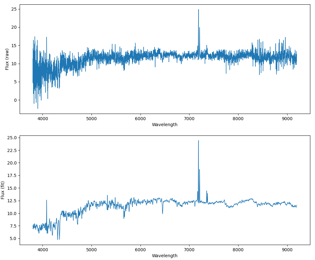
Now, we plot both flux and model on y-axis and wavelength on x-axis.
fig, ax = plt.subplots(2, 1, figsize=(12,10))

ax[0].plot(wavelength, flux, linewidth=1)
ax[1].plot(wavelength, model, linewidth=1)

ax[0].set_xlabel('Wavelength')
ax[1].set_xlabel('Wavelength')
ax[0].set_ylabel('Flux (raw)')
ax[1].set_ylabel('Flux (fit)')

plt.show()
The emission lines
Up to here, we have just worked with the first extension of the FITS file. The second extension just gives us some general information, such as coordinates, class of object, redshift, etc. Most of these could be requested by SQL scripts directly from the SDSS servers, so we don’t explain them here.
The third extension is important for our project. This is where the information about emission lines can be found. In fact, the plot of a spectrum without indication of spectral lines doesn’t give us much information. Let’s see column names of the third extension:
cols3 = hdul[3].columns
data3 = hdul[3].data

print(cols3)
ColDefs(
    name = 'PLATE'; format = 'J'
    name = 'MJD'; format = 'J'
    name = 'FIBERID'; format = 'J'
    name = 'LINENAME'; format = '13A'
    name = 'LINEWAVE'; format = 'D'
    name = 'LINEZ'; format = 'E'
    name = 'LINEZ_ERR'; format = 'E'
    name = 'LINESIGMA'; format = 'E'
    name = 'LINESIGMA_ERR'; format = 'E'
    name = 'LINEAREA'; format = 'E'
    name = 'LINEAREA_ERR'; format = 'E'
    name = 'LINEEW'; format = 'E'
    name = 'LINEEW_ERR'; format = 'E'
    name = 'LINECONTLEVEL'; format = 'E'
    name = 'LINECONTLEVEL_ERR'; format = 'E'
    name = 'LINENPIXLEFT'; format = 'J'
    name = 'LINENPIXRIGHT'; format = 'J'
    name = 'LINEDOF'; format = 'E'
    name = 'LINECHI2'; format = 'E'
)
Here, we are specially interested in four of these columns: LINENAME, LINEWAVE, LINEZ and LINEAREA. These are the names of the lines, the rest wavelengths of the lines, the calculated redshift from each line, and areas of the lines, respectively. Let’s extract these columns in four new variables and create a pandas DataFrame from them:
line_names = data3.field('LINENAME')
line_waves = data3.field('LINEWAVE')
line_z = data3.field('LINEZ')
line_area = data3.field('LINEAREA')

df = pd.DataFrame(
    {'name': [i for i in line_names],
     'lam_rest': [i for i in line_waves],
     'z': [i for i in line_z],
     'area': [i for i in line_area]
     }
    )

df = df[abs(df['area'])>0]
print(df)
             name     lam_rest         z       area
6     [O_II] 3725  3727.091727  0.094871  30.996830
7     [O_II] 3727  3729.875448  0.094871  24.527514
8   [Ne_III] 3868  3869.856797  0.094871  -3.518241
9       H_epsilon  3890.151080  0.094871  -8.486563
10  [Ne_III] 3970  3971.123187  0.094871 -22.393383
11        H_delta  4102.891631  0.094871  -6.722156
12        H_gamma  4341.684313  0.094871   3.061384
13   [O_III] 4363  4364.435300  0.094871   1.015044
14     He_II 4685  4686.991444  0.094871  -1.985071
15         H_beta  4862.682994  0.094871   9.303711
16   [O_III] 4959  4960.294901  0.094870   6.017811
17   [O_III] 5007  5008.239638  0.094871  18.227947
18     He_II 5411  5413.024423  0.094871  -2.460578
19     [O_I] 5577  5578.887704  0.094872  -1.581697
20     [O_I] 6300  6302.046377  0.094872  10.753190
21   [S_III] 6312  6313.805533  0.094870   0.442675
22     [O_I] 6363  6365.535420  0.094871   4.292485
23    [N_II] 6548  6549.858929  0.094871  15.137597
24        H_alpha  6564.613894  0.094870  83.739006
25    [N_II] 6583  6585.268445  0.094870  54.291546
26    [S_II] 6716  6718.294208  0.094871  23.901695
27    [S_II] 6730  6732.678076  0.094871  12.859660
28  [Ar_III] 7135  7137.757103  0.094871  -1.571996
We have deleted the rows whose line areas were zero because we don’t need them. Note that the wavelengths of the lines are rest or emitted wavelengths. These are the values that we already know from the laboratories on the Earth. But in the spectrum we should draw the observed wavelength of lines. According to the definition of the redshift:
![\[ z = \frac{\lambda_{obs}-\lambda_{rest}}{\lambda_{rest}} \]](https://astrodatascience.net/wp-content/ql-cache/quicklatex.com-792b6b3a940f5119dc1f91804ea0d083_l3.png "Rendered by QuickLaTeX.com")
So,
![\[ \lambda_{obs} = \lambda_{rest}(1+z) \]](https://astrodatascience.net/wp-content/ql-cache/quicklatex.com-ab1539bd4da6ce96727704f4daed2c99_l3.png "Rendered by QuickLaTeX.com")
Using the above formula, we can calculate the observed wavelength of the lines easily:
df['lam_obs'] = df['lam_rest'] * (1 + df['z'])
Now we are ready to create the plot of the spectrum.
fig, ax = plt.subplots(figsize=(12,8))

label_y = np.random.uniform(
    low=model.min().value*1.1,
    high=model.max().value*0.9,
    size=len(df)
    )

ax.plot(wavelength, model, linewidth=1)

for i in range(len(df)):
    ax.axvline(x=df['lam_obs'].iloc[i],
               color='r',
               alpha=0.3,
               label=df['name'].iloc[i],
               ls='--',
               lw=0.7)

    ax.text(x=df['lam_obs'].iloc[i] ,
            y=label_y[i],
            s=df['name'].iloc[i],
            fontsize='small',
            rotation=90)

plt.xlim(4000, 8000)
plt.show()
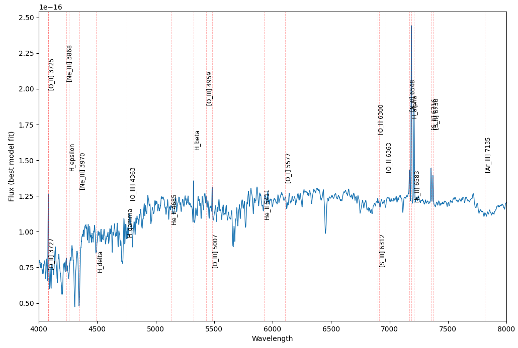
Not bad. But the problem is that when the line are so close to each other they can not be distinguished. This is why we need an interactive plot that can be zoomed in and out.
Making the plot interactive
In order to create an interactive plot we use bokeh python package. There are also other libraries such as plotly that could be used in the same way. First, we should import necessary libraries and create the plot in almost similar way. Here, we can use some features such as hover tools that let’s the user to view some useful information.
from bokeh.plotting import figure, show
from bokeh.models.tools import HoverTool
from bokeh.models import Span, Label

p = figure(title="Spectrum",
           sizing_mode="stretch_width",
           x_range=(4000, 8000),
           tools=[HoverTool(), 'pan', 'wheel_zoom', 'reset'],
           tooltips="lambda=@x{0.000} | flux=@y",
           x_axis_label="Wavelength", y_axis_label="Flux")

p.line(wavelength, model, line_color="blue", line_width=1)

for i in range(len(df)):
    ver = Span(location=df['lam_obs'].iloc[i],
               dimension='height',
               line_color='red',
               line_dash='dashed',
               line_width=1)

    p.add_layout(ver)

    lbl = Label(x=df['lam_obs'].iloc[i],
                y=label_y[i],
                text=df['name'].iloc[i])

    p.add_layout(lbl)

show(p)
You can find the complete source code here.