Hubble’s Law

Hubble Constant

In 1929 Edwin Hubble published an article in which he presented empirical evidence that our universe is expanding. At that time, most of the scientists believed in a static universe. After publishing Hubble’s article, Einstein called the assumption of static universe his biggest mistake. He went to Mount Wilson Observatory to thank Hubble for his great discovery.

In this article, Hubble presented a linear relationship between distance and radial velocities of a number of galaxies. This relation, which is known as Hubble’s Law, is represented as follow:

In this formula, is the radial velocity, is proper distance and is Hubble constant. It states that galaxies are moving away from each other at a speed proportional to their distances. In other words, the farther a galaxy is from us, the faster it is moving away from us.

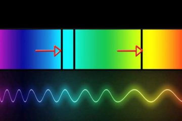
Hubble used a sample of galaxies whose distances where known. Instead of radial velocity, he used redshift. We know that , so knowing the redshift of a galaxy, we can find its radial velocity simply by multiplying redshift by speed of light.

Now I’m going to do exactly what Hubble did in his famous article. You can find the sample used by Hubble as a CSV file here. Let’s load the dataset and see a few rows of it.

>>> import pandas as pd
>>> data = "https://github.com/behrouzz/astrodatascience/raw/main/data/hubble1929.csv"
>>> df = pd.read_csv(data)
>>> print(df.head())
     galaxy  distance  velocity
0     S.Mag     0.032       170
1     L.Mag     0.034       290
2  NGC.6822     0.214      -130
3   NGC.598     0.263       -70
4   NGC.221     0.275      -185

For not being confused, let’s use x for representing distance and y for representing radial velocity. We are going to find the slope of the line , which is . The polyfit function from numpy do this for us:

>>> import numpy as np
>>> x = df['distance']
>>> y = df['velocity']
>>> slope, intercept = np.polyfit(x, y, 1)
>>> print(slope)
454.1584409226285

As you see slope is about 454. Let’s first plot the dataset points and the regression line and then explain it.

import matplotlib.pyplot as plt

fig, ax = plt.subplots()
ax.scatter(x, y, color='blue')
ax.plot(x, slope*x + intercept, color='red')
ax.set_xlabel('Distance (Mpc)')
ax.set_ylabel('Recessional Velocity (km/s)')
plt.grid()
plt.show()

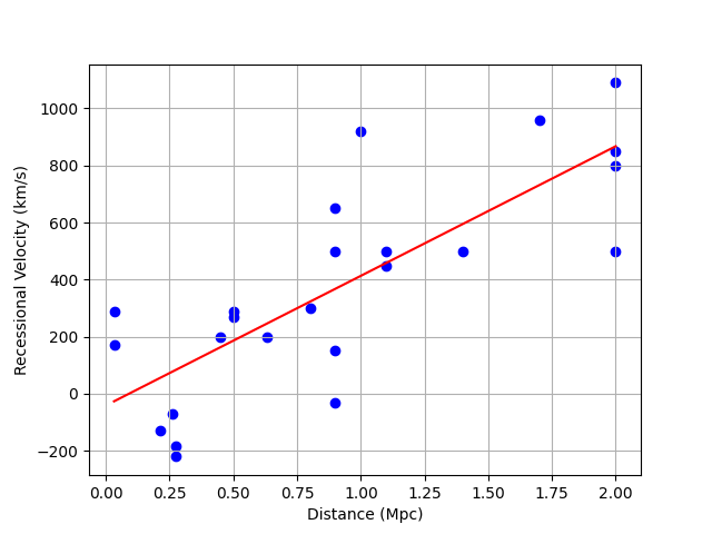
Note that the unit of distance is and the unit of radial velocity is . So, the unit of should be . The resulting formula should be . It means that if a galaxy is at 1 away from us, it is moving away from us at speed of 454 . The method used by Hubble was correct, but the number he calculated for was NOT correct.

In fact, the expansion of the universe applies only on large scales. By large scale, we mean distances more than 100 . In short scales, the expansion of the universe does not have any effect on gravitational bounded structures. For example, distances between the stars in our galaxy do not increase by the expansion of the universe. The galaxies sample used by Hubble were all galaxies whose distances were less than 2 Mpc. The major problem in calculating Hubble’s constant is the way the distances should be estimated. It was not a simple task in 1920s to calculate distances more than 100 Mpc.

Let’s now calculate using a simple and powerful tool created by Centre de données astronomiques de Strasbourg. SIMBAD is a database that contains data from a lot of different astronomical catalogs. The most efficient way to retrieve data from this database is using SQL scripts. You can type your scripts directly in the TAP Service page or you can use hypatie python package to retrieve data.

We’re going to use two tables from SIMBAD database: basic and mesDistance. We join these two tables to retrieve distance and redshift for a sample of 1000 galaxies whose distances are higher than 100 Mpc. In order to prevent getting distances in the database which have been estimated from redshift, we need to indicate the method used to calculate distance. In the following SQL script, we’ve chosen T-F method.

from hypatie.simbad import sql2df
import numpy as np
import matplotlib.pyplot as plt

sql = """
SELECT TOP 1000 
b.rvz_redshift AS z, d.dist AS D
FROM basic AS b
JOIN mesDistance as d ON b.oid=d.oidref
WHERE dist > 100 AND unit='Mpc' AND method='T-F'
AND rvz_redshift BETWEEN 0 AND 0.1
"""

df = sql2df(sql)
df = df.astype('float')

# Calculate radial velocity
df['v'] = 299792.458 * df['z']

# Calculate H0
x = df['d']
y = df['v']
slope, intercept = np.polyfit(x, y, 1)

# Plot data and regression line
fig, ax = plt.subplots()
ax.scatter(x, y, color='blue', s=1)
ax.plot(x, slope*x + intercept, color='red')
ax.set_title('Calculated H0: '+str(round(slope,2))+' (km/s)/Mpc')
ax.set_xlabel('Distance (Mpc)')
ax.set_ylabel('Recessional Velocity (km/s)')
plt.grid()
plt.show()

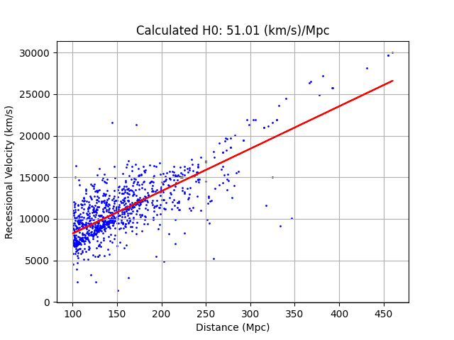
The value we calculated, 51.01, is much more realistic than that calculated by Hubble. According to Planck Mission final results, released in 2018, which is higher than what we calculated.

Hubble Parameter

The Hubble constant , as we’ve seen, is a proportionality constant that relates distance to radial velocity. But the value of describes the relationship between these two quantities only at the present day. In fact, slope of the regression line in the above diagrams changes with time. This slope is called Hubble parameter, denoted by , which is a function of time. Thus, the Hubble constant is just the value of at the present day.

The Hubble parameter can be written in terms of scale factor:

In this formula, is scale factor, which is a function of time, and is time derivative of scale factor.

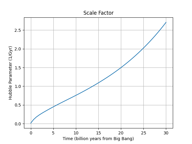
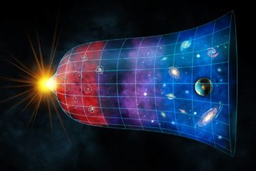
Let’s try to plot the diagram of scale factor and Hubble parameter to find out how the geometry of our universe changes with time. I’ve written another post explaining how to calculate scale factor, but if you are not interested in the details of calculation, you can simply use the function scale_factor from hypatie. We create an instance of Planck18 class as our cosmological model. Then we use its scale_factor method which gives us the scale factor as a polynomial function. By creating a range of time points and passing them to the scale factor function, we can find for each moment of time its corresponding scale factor. Note that the scale_factor method needs the time passed to it to be in billion years starting from the Big Bang.

import numpy as np
import matplotlib.pyplot as plt
from hypatie import Planck18

cosmo = Planck18()
a = cosmo.scale_factor()
t = np.linspace(1e-10, 30)

plt.plot(t, a(t))
plt.title('Scale Factor')
plt.xlabel('Time (billion years from Big Bang)')
plt.ylabel('Hubble Parameter (1/Gyr)')
plt.grid()
plt.show()

For calculating the Hubble parameter, we should create a function by dividing time derivative of scale factor to scale factor. This is a function of time, so, if we give it a moment, it gives us the value of the Hubble parameter at that moment. As we’ve said before, the value of the Hubble parameter at the present day is the Hubble constant, . Let’s see what our function gives us if we pass the current age of the universe:

>>> def H(t):
	return a.deriv(1)(t) / a(t)

>>> H(13.8)
0.06933802993205697

The result, 0.069, is . What does it mean? It means that at the current rate of the expansion, the universe expands about %7 each one billion years. But why is it so different with values we saw before, like 51 or 67? Because its unit is in . Let’s convert it to the conventional unit . If you are lazy in converting units, like me, use astropy.unit module:

>>> from astropy import units as u
>>> x = (1*u.Unit('1/Gyr')).to('km / (Mpc s)')
>>> print(x)
977.7922216807892 km / (Mpc s)

So, each unit of equals 977.792 units of . Let’s convert H to the conventional unit and name the new function H_conv and see what it gives us if we pass the current age of the universe:

>>> def H_conv(t):
	return 977.7922216807892 * H(t)

>>> print(H_conv(13.8))
67.79818633423504

As you see, the result is now reasonable. Finally we plot it:

>>> plt.plot(t, H_conv(t))
>>> plt.title('Hubble Parameter')
>>> plt.xlabel('Time (billion years from Big Bang)')
>>> plt.ylabel('Hubble Parameter (km/s)/Mpc')
>>> plt.ylim(0, 300)
>>> plt.grid()
>>> plt.show()

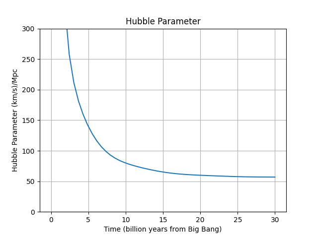
Well, you can see the Hubble parameter is decreasing with time. What does it imply? Remember the Hubble’s Law and imagine yourself as an observer on the Earth who are looking at a point at a fixed distance far away from the Earth. You see galaxies pass this point at velocity . After billion years, the Hubble parameter will be and you see galaxies passing that point at speed . Since the Hubble parameter is decreasing, , you will see that the later galaxies pass the fixed point at lower speed: .

Be careful not to confuse the accelerating rate of the expansion with the decreasing trend of the Hubble parameter. The expansion of our universe is now accelerating, because the second derivative of scale factor is positive at the present day. You can check it simply by pass the current age of the universe to the second derivative of scale factor:

>>> a.deriv(2)(13.8)
0.0023715549918029155

As a final word, I should say that one important role of the Hubble parameter is that it appears in the Friedmann equation, which relates the distribution of energy density to the geometry of the universe.